Saturday, December 22, 2012

SSAS - Designing approaches for dimensional model


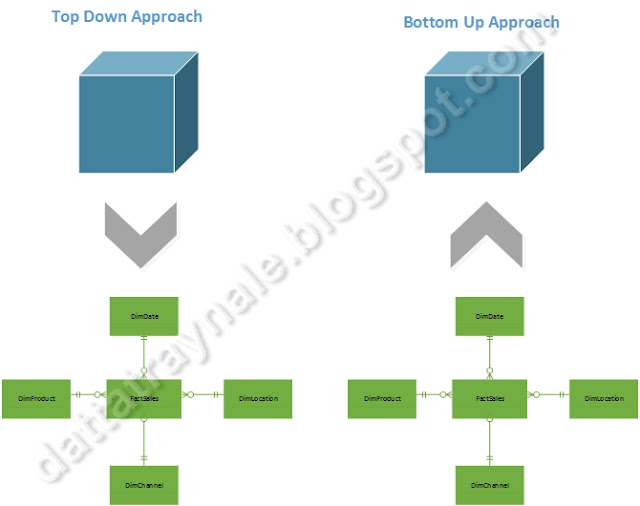
In SSAS, there are two ways to design dimensional models. Top-down or bottom up.

Top Down Approach
  • This is generally not much used option.
  • The relational data source does not exist in this case. The tables are created from the dimensional model from SSAS.
  • Cube and dimension wizards has the option to implement this option.
  • Schema Generation Wizard is used to generate and deploy schema in the database..
  • DBO permission required in order to create database objects.

Bottom Up Approach
  • Most of the times this is the approach thats taken.
  • The data mart already exists.
  • The dimensional model and cubes are designed from the Relational tables in the Data Mart.
  • Cube and Dimension wizards have the option to implement this solution.
 

Monday, December 10, 2012

SQL Server - Cost estimation issues even with up-to-date statistics

The only way to know if statistics are update-to-date or outdated is look at Actual Records count and Estimated Records count in an execution plan. A mismatch indicates that statistics need to be updated. But there are exceptions to this rule. There are situations when even if statistics is up-to-date still there is a difference in estimated and actual count.


First let's check the result with fixed parameter query. In my example I have bloated the data in AdventureWorksDW2008R2.FactInternetSales by duplicating the data multiple times (of couse, ensuring that the Primary key is unique).

T-SQL with fixed query (OK)


T-SQL with local variables (Issue)


Stored procedure with local variables (Issue)

 Here are the scenarios when the same query with different implementation style would give a matching estimated and actuals count.


Possible Solutions...

Here are the possible solutions to correct the issue.
    Stored procedure without local variables (OK)


    Dynamic sql with sp_executesql (OK)


Dynamic sql with EXEC (OK)


_

Saturday, December 1, 2012

Big Data - 1: A big picture


Everyday we get bombarded with terminologies in connection with big data like NoSQL, RavenDB, Hadoop, MongoDB and so on. Since this is an upcoming area in IT, we struggle to understand what those terms are and how these technologies can help us. I am not an expert in Big data, but I would share what I have known so far.


The diagram above gives a high level view of various terminologies in the big data arena and their relationship with each other.
  • Big Data : 
    • Big data is the data that is big in terms of
      • Volume (terabytes, petabytes and above)
      • Velocity (rate of transmission and reception) 
      • Variety (complexity, text, pictures, videos etc).
    • Big data by itself is messy and would not make any sense as it is unstructured or semi-structured unlike traditional data. The only way it can be useful is pull out only the relevant information. Pulling out relevant information out of such big data is the real problem that traditional sytems cannot help in. This is where big data technologies come into picture
There are three technology classes that support Big Data. Hadoop, NoSQL and Massively Parallel Processing (MPP) databases. I would start with MPP databases as they have been there for decades.
  • MPP Databases: These databases spread the data into independent storage and CPU thus achieving parallellism and great processing capability. This is special hardware and software combination that help you achieve such parallellism. The big products in market are IBM's Netezza, HP's Vertica and EMC's Greenplum. Microsoft's SQL Server Parallel Datawarehouse (PDW) is one upcoming MPP database.
  • Hadoop : Hadoop is one of the technology classes that support big data. It is an opensource version of Mapreduce created by Apache software foundation. In general, Mapreduce is parallel programming framework.
  • NoSQL : NoSQL stands for "not only SQL". It represents a class of databases that do not follow RDBMS principles (like transactional integrity) and mainly deal with big data. There are four categories of NoSQL databases. Please refer to the diagram above for the database products that fall under the below categories. Few of the NoSQL databases work in conjunction with Hadoop components.
    • Document store
    • Graph Database
    • Key-Value store
    • Wide Column store
I hope this post was useful in understanding the basic terminologies of big data and related technologies.

 In the next big data post, I would provide more details on NoSQL database categories.

Monday, November 26, 2012

SQL Server - Partitioning Design : 4 - Partitioned Tables + Partitioned View

This post is an extension to the previous post - Partitioning Design Patterns. In order to understand this post, you would need to go through the previous post. In this post I will write in-depth on why this design is an optimal solution. I would cover only those points that make this design a preferred implementation style as compared to other designs.


How this works?

  • Please refer to the diagram above.
  • Data for each year stored in separate physical table. In the above example, FactTransaction_2010, FactTransaction_2011, FactTransaction_2012, FactTransaction_2013.
  • Each physical table is partitioned into one partition per month.
  • Each table is stored on a different file group. Each file group having 4 files per filegroup.
  • Each filegroup is stored on a different storage drive based on workload. More recent data (very frequently accessed) is stored on high performance storage option. Older data generally accessed less frequently is placed on a less performance, less expensive storage option.
  • A view (FactTransaction_vw, union All on all tables) exposes the data in all the tables. The application queries uses this view for its reporting needs.
  • A synonym (FactTransaction_syn) points to the underlying table that is for current year (FactTransaction_2012). All the queries that insert or update data for current year, would use the synonym. Next year, the synonym would be pointed to the relevant table without any impact on existing code.
  • Most imporantly, tables for each year will have a check constraint on the date column (Partition column) for valid date range. For example, a check constraint on date column in FactTransaction_2012 to ensure that data from 1Jan2012 to 31Dec2012 can be stored. With this sql server does table elimination when searching for a particular date. Since each table is further partitioned per month, SQL Server does partition elimination. For instance, if a user queries data for 10 Nov 2012. SQL Server would directly jump to table FactTransaction_2012 (Table elimination. Check constraint helps sql server do this) without going to any other table and then within FactTransaction_2012 it jumps to partition meant for month Nov (partition elimination). This greatly helps in partition column based search operations.

Variations of this design depending on data volume


       With some more creativity, this design can be tweaked if daily/monthly data volumes are too heavy. But do a thorough testing if this really works for you. Below is one such variation.
    • One table for each year (FactTranaction_2010, FactTransaction_20xx, and so on).
    • Each table relevant to each year can be partitioned per month (or even date).
    • One separate table (FactTransaction_CurrentMonth) that would store data for current month (or quarter depending on data volume).
    • Daily rebuilds could to be done only on FactTransaction_CurrentMonth  table which would be a very small fraction of a huge historic table. Any maintenance activity like index rebuild or statistics update would not put undue pressure on system resources and would definitely benefit the system availability.
    • Once current month is done (Eg Nov2012), the current month data from FactTransaction_CurrentMonth can be merged in the FactTransaction_2012 table. Then FactTransaction_CurrentMonth would be used to store Dec2012 data and so on.
    • Monthly rebuilds need to be done on Yearly table after merging current month data from FactTransaction_CurrentMonth to FactTransaction_2012.

Pros

Below benefits give this design an edge over other implementations. Please remember, I have not mentioned all other benefits of this design that overlap with other designs.
  • Relieves SQL Server from unwanted CPU and IO pressure from online/offline index rebuilds.
    • Index rebuild is something that cannot be avoided by any database implementation. Based on index design and index fragmentation levels, indexes might need to be rebuilt as a part of daily batch. Index rebuilds are generally a problem for huge databases due to space requirements and resource consumption.
    • Let's understand this with an example. Let's say there is a table with 1 Terabyte (TB) of data. This table stores 4 years of data. If any partitioning design pattern except Design-4 is implemented, then index rebuild would lead to a very big hit on CPU and IO. In case of clustered index, because it includes actual data pages plus other index pages; the clustered index size would be 1 TB (data size) + other index pages size. Rebuilding such a clustered index is going to be a huge spike on server in terms of IO and CPU consumption. In case of non-clustered indexes, even if it does not contain the data pages as in case of clustered index; its still going to hit CPU and IO as well. That's because, the Non-clustered index structure will store data for all the historic data of entire table. Let's say, there are 5 non-clustered indexes, and each index is (hypothetically, based on design) is 100 gb. So a rebuild here will lead to rebuild of 500 gb of data which will lead to a big hit on server resources.
    • It's worth a thought... why should the index data for previous years be rebuilt over and over again, even if what really needs to be rebuilt is only current year data. Now coming to the recommended multiple table based design, data is already split into multiple "separate" physical structures. Obviously, rebuilding only the current year indexes will be very light on SQL Server as compared to rebuilding indexes on a single table with all the historic data
 
  • Better availabiliy with online rebuilds.
    • A particular partition can be rebuilt only in offline mode. Online option is available only for entire table. This can be an issue for applications that need to be online 24x7. In offline mode, the partition being rebuilt is not available for querying.
    • With a table for each year, the entire data is divided into separate structures and so rebuilding only a single year table becomes more practical in ONLINE mode.
    • If a single year data is huge, the solution can be tweaked to suit your needs. Refer to section "Variations of this design depending on data volume". As mentioned in the example, online rebuild would take very small fraction of time, as only a very small fraction of data would be rebuilt. For example, in the FactTransaction_CurrentMonth, on day-1 only one day data would to be rebuilt. On Day-2, two days and so on until day 31. So at the max 31 days of data would be rebuilt, while rest of the data for all the years is untouched. That cuts down a lot of maintenance time and resources and enhances application availability.

  • Space issue associated with online rebuilds is eradicated.
    • Rebuilding indexes in online mode on huge tables need a lot of space. Any many a times, the rebuilds fail due to lack of space. Let's understand this with an example.
    • For instance, if a clustered index on table with 500 GB data needs to be rebulit, it would need 1.1 Terabyte of space. This is how it would need.
      • A copy of data is created which would need 500 GB
      • Around 20% of sorting space, that would be 100 GB
      • 500 GB of log is generated.
      • If mirroring is implemented, then it would generate a lot of network traffic.
    • Lets see the space requirement with this design or its variation (FactTransaction_CurrentMonth). For instance, the FactTransaction_CurrentMonth table that stores one month of data at the max would store 10 GB at the end of the month. At the max it would need around 22 GB of space.
      • A copy of data is created which would need 10 GB
      • Around 20% of sorting space, that would be 2 GB.
      • 10 GB of log is generated.

  • Relieves SQL Server from unwanted CPU and IO pressure from statistics recompute for a huge base data.
    • A huge table will have huge regular indexes. There could be situations when the performance is bad due to skewed statistics as the sampling size is not enough. Scanning such huge data with higher sampling size to rebuild statistics would overkill CPU and IO for a long time, as sql server has more data pages to scan through to create more accurate statistics.
    • With one huge table storing data for all the previous years, statistics update would lead to re-computation of statistics for all the previous years. This is un-necessary work. Would it not be great if only current year statistics is being recomputed. Previous year statistics can be computed once and used multiple times by all the queries.

  • Helps SQL Server in maintaining accurate statistics which is a major contributor in better query performance.
    • Apart from the undue pressure on CPU and IO, huge tables also lead to skewed statistics. The rule is, small tables have accurate statistics and huge tables by default have skewed statistics. In this particular design, because each table is a separate physical structure, the statistics too are maintained separately for each table by year. If it was one big table with all the historic data, there would be huge statistics maintained for that table.
    • So why accurate statistics are beneficial for better execution plans? Thats because accurate statistics have enough data to help sql server come up with a good execution plan. If the statistics is skewed, SQL Server cannot come up with good execution plan. This follows the standard rule - "Garbage in, garbage out".
    • Since this blog is not dedicated to statistics, I cannot include more details on why and how statistics get skewed on huge tables. I would do that in a separate post. But in general stats get skewed in huge tables because SQL server computes statistics only on occurence of certain events and when it does, it uses a sampling algorithm. The samples might not be enough to compute accurate statistics

Cons    

  • Any change in table schema need to be reflected in all the underlying tables. If you have 10 tables for 10 years, then all those would need to be updated with the new schema. Although there is another way to avoid this. One can create a dummy value column in the view. But I would not prefer that as a personal choice.
  • Can have max of 255 tables in a view. This practically should not be an issue as it would mean 255+ years of historic data which is next to impossible for all practical purposes.

Please leave your comments if you liked/have suggestions for  this blog post.


Sunday, November 25, 2012

SQL Server - Wait Statistics : 2 - SQL Server Thread and Task Architecture


  • Each Physical CPU has one or many mapped Logical CPUs. A Logical CPU has to have one and only one mapped Physical CPU.
  • One scheduler is assigned to one Logical CPU. However, a logical CPU can have multiple schedulers.
  • A scheduler maintains two structures, Runnable queue and Wait list. Runnable Queue is maintained for the collection of Runnable tasks. As Queue is a First in First out operation, the first task in the queue waiting for CPU time will be executed first and then the second in the queue.The Wait/Suspended List is an un-ordered set of tasks waiting for some resource. Once the resource is available, the task is pushed to Runnable Queue. So the task in Wait list waits until the resource the task is waiting for is available.
  • A scheduler (logical CPU) is assigned a set of workers (Thread or fiber depending on configuration) to execute tasks.
  • If you pause and think about the previous 4 points, it becomes logical that each logical CPU or scheduler would maintain its own Runnable Queue and Wait List. And since each logical CPU is an independent CPU for SQLOS, each Logical CPU/Scheduler has its own work and task assigned to it. And thus multiple CPUs would lead to parallellism.
  • The worker is bound to the task until its finished. This means if for some reason the task is suspended due to unavailable resources, the worker too waits. The worker is assigned a new task only when it finishes the current task in context.
  • At a given point of time, a task can be in either in Runnable, Suspended or Running state. It may change the state in the below fashion
    • Running >> Suspended >> Runnable >> Running
While a task is running, it might need a resource (data page, memory, lock etc)
which might not be available. If the resource is unavailable, then the task is changed
to Suspended state. And it remains there until it gets the resource its waiting for.
Once the resource is available the task is moved to Runnable state. This means that
the task is ready to be processed and it waiting in Queue for the processor time. It
gets executed once the tasks before it in the queue are executed.
    • Running >> Runnable >> Running
While a task is running, it might directly enter into a runnable state without going in
suspended state. This will happen if the task meets its quantum exhaustion. A
quantum exhaustion is the time limit a task can use processor time.
In SQL Server its 4 milli seconds. This means after 4 milli seconds, the current task
will be pushed to the bottom of runnable queue and the task on the top of the queu
will be popped for processing.
Tuesday, November 20, 2012

SQL Server - Find number of physical processors, cores, logical processors and RAM using T-SQL


There are times when you want to know the SQL Server box configuration, specifically processors. It can be frustrating if you have to wait for a couple of days for another group in your ogranization to give the information. Here is something, that you can use to find out the details yourself.

I found many posts that help you find physical and logical CPUs. But I was interested specifically in the number of cores too. Few posts mentioned that there is no way you can find number of cores using T-SQL.

Here is the query that can give you the number of cores too. Test it yourself and let me know if this does not work in your scenario.

SELECT ( cpu_count / hyperthread_ratio )AS NumberOfPhysicalCPUs
, CASE
WHEN hyperthread_ratio = cpu_count THEN cpu_count
ELSE ( ( cpu_count - hyperthread_ratio ) / ( cpu_count / hyperthread_ratio ) )
END AS NumberOfCoresInEachCPU
, CASE
WHEN hyperthread_ratio = cpu_count THEN cpu_count
ELSE ( cpu_count / hyperthread_ratio ) * ( ( cpu_count - hyperthread_ratio ) / ( cpu_count / hyperthread_ratio ) )
END AS TotalNumberOfCores
, cpu_count AS NumberOfLogicalCPUs
, CONVERT(MONEY, Round(physical_memory_in_bytes / 1073741824.0, 0)) AS TotalRAMInGB
FROM
sys.dm_os_sys_info
 
 Please keep in mind, you need to have VIEW SERVER STATE permission to use the DMV sys.dm_os_sys_info 


Monday, November 19, 2012

SQL Server - Wait Statistics : 1 - SQL Server Operating System (SQLOS) Basics

Few basic concepts around SQLOS which is a core component in SQL Server architecture, are critical for understanding SQL Server behaviour. If one wants to be good at troubleshooting performance issues in SQL Server, these concepts would help in creating that solid foundation. This blog is intended to explain the details around SQLOS and wait statistics in a simplified form. The entire topic will be covered in a series of posts. 

Let's go through these terms before we dive deep.
  • SQLOS can be visualized as a mini operating system built for SQL Server that works on the top of Windows Operating system. This Operating system works on the top of Windows OS to help SQL Server perform some critical functions. This means that SQLOS in many cases can also be dependent on Windows OS. SQLOS was first introduced in SQL Server 2005. In general, SQLOS performs two major functions of scheduling and memory management.
  • Physical CPU can be a multicore or single-core CPU on the SQL Server box. Each core acts as an individual processor. For example: a quad core cpu means on a single die, there are 4 CPUs.
  • Logical CPU is CPU visible to Operating System (OS) irrespective of number of physical CPUs for its processing needs. There could be a quad core physical CPU (4 physical CPUs); but with the help of technologies like hyperthreading double the number of physical CPUs (i.e. 8 CPUs) are exposed to OS.
  • Scheduler is a logical CPU on SQL Server side. Each scheduler is mapped to one logical processors exposed by operating system. However, one logical processor can have multiple schedulers assigned to it. Schedulers can be visible or hidden. A visible scheduler is visible to SQL Server user processes, whereas, the hidden scheduler is visible only to SQL Server internal processes. One scheduler is dedicated to DAC (Dedicated admin connection). This DAC is a back entry to SQL Server for the DBA if the server hangs.
  • Worker is something that executes a task. Scheduler is also called worker thread. Worker threads in SQL Sever are mapped to windows threads or fibers by scheduler.
  • Task is a unit of work assigned to SQL Server. Generally a session submits a batch. This batch is broken into multiple tasks and these are processed by multiple threads. This leads to parallellism.
  • Session or SPID is a connection over which requests are sent to SQL Server.

Wednesday, November 14, 2012

SQL Server - partitioning design patterns

      Before jumping to the topic of partitioning design patterns, I would brush up on the basic concepts of partitioning.

What is Partitioning?
  • In general, partitioning  means breaking “something” into manageable pieces.
  • From database point of view:
    • Functionality to horizontally split the table while maintaining a single logical object.
    • This can a feature coming with a DB product, or it can be designed to achieve the same functionality.
  • There are two types of database partitioning that can be implemented by partitioning a table vertically or horizontally.
 
Partitioned Table


Why Partition?

So what are the situations when one would need to consider partitioning?
  • One or more tables would grow around 40+ GB.  And that will lead to the issues below…
  • Query processing performance is a concern.
  • DBA operations like index rebuild, statistics update, backups, restores, recovery are time consuming (Availability issues)
  • Slow Data Load / Archive / Delete operations

Limitations of Partitioned Tables
  • A specific partition can be rebuilt only offline (Restriction). This is an issue for global applications.
  • Online index rebuild takes ages in monster tables. That also leads to multiple other problems.
    • System performance is impacted during online rebuild
    • Extra space : table with 500 GB data, Clustered Index rebuild needs 1.1 TB space (500 GB  data part + 100 GB sorting space + 500 GB log generated)
       Apart, mirroring traffic (if mirroring implemented). If this space is not available, then indexes cannot be rebuilt.
    • Resource abuse : rebuilding static part of data, when it can be done once.
  • Skewed/Inaccurate statistics leading to performance issues.
     
Partitioning Solution

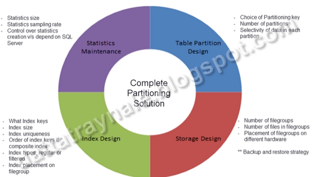
    Partitioning implementation might look like an easy implementation, but its really a complex process. Just knowing partitioning feature is not enough to come up with a really performing partitioning solution. The scope of a partitioning solution is much bigger that I have tried to put in the diagram below. The design decisions that need to be taken in each area are listed in the bulletted points next to each quadrant. Wrong decisions in these areas will lead to poorly implemented partitioning solution. Which means, the person who is responsible for this implementation should also know other internal aspects of SQL Server. This diagram can be seen as a check-list for such implementation.


Partitioning Design Pattern:1 (Basic)


Cons
  • Specific partition can only be rebuilt in offline mode.
  • Online index rebuilds take long, impacting the application performance.
  • Index rebuild may fail due to DB space issues.
  • Statistics issues – stats invalidation takes longer in big tables, skewed statistics, stats rebuild with full scan drains out resources.
  • Takes longer to backup and restore.
  • Piecemeal restore not available due to single filegroup.
  • High storage costs.
This solution is not recommended
-------------------------------------------------------------
Concepts
Benefits of multiple filegroup based design
  • Cost Effectiveness : More actively used data placed on high perf hardware (e.g. Solid state drive/Raid 10) and less frequently accessed in less expensive/low performing hardware.
  • Narrow maintenance window : File/File groups help piecemeal data backups and restores. Static data need to be backed only once, leading to Storage costs reduction (SAN is expensive).
  • Better Availability : Partial database recovery is possible. More important/actively used data can be brought online soon. In case of file corruption only the impacted filegroup is not available.
-------------------------------------------------------------
Design Pattern:2 (Non aligned Partition Indexes)
Pros
  • Parallel access to indexes and data 
Cons
  • Specific partition can only be rebuilt in offline mode.
  • Online index rebuilds take long, impacting the application performance.
  • Index rebuild may fail due to DB space issues.
  • Statistics issues – stats invalidation takes longer in big tables, skewed statistics, stats rebuild with full scan drains out resources.
  • If index filegroup gets corrupted/offline, then the entire    table is in accessible.
  • Partial database recovery can be implemented, but less efficient and not a clean solution.
This solution is not recommended

Design Pattern:3 (Partition aligned regular indexes)

Pros
  • Partitioned table advantages.
 Cons
  • Specific partition can only be rebuilt in offline mode.
  • Online index rebuilds take long, impacting the application performance.
  • Index rebuild may fail due to DB space issues.
  • Statistics issues – stats invalidation takes longer in big tables, skewed statistics, stats rebuild with full scan drains out resources.
  • Partial database recovery possible but not a clean solution
This is a generally implemented solution but I would not recommend this solution unless fully justified.

-------------------------------------------------------------
Concepts
 Partitioned View


Advantages of partitioned views based design
  • Table Elimination for query performance. This can be achieved by adding a check constraint in table for every year on the partition Column (Eg date).
  • Different indexes can be created on underlying tables. For instance, index based on access patterns, different fill factors etc. based on usage.
  • Statistics is not/less skewed. More accurate stats lead to better execution plans, thereby better performance.
  • Stats update operations need to be done only for current year. Previous years are untouched. Huge reduction in maintenance window.
  • Online index rebuild is supported for an entire table for a particular data set. Other static data need not be rebuilt. This will save space requirements just to rebuild large indexes, which translates to more cost.
  • Not required data can be deleted in micro-milli-secs, by dropping the table itself and updating the view.
-------------------------------------------------------------